In today's volatile capital markets, presenting a single-point discounted cash flow (DCF) valuation has become professionally insufficient—and potentially misleading. With interest rates fluctuating between 4.5% and 5.5% throughout 2024-2025, equity risk premiums expanding to 6.2-7.8% across developed markets, and terminal growth assumptions under constant scrutiny, sophisticated investors and boards demand comprehensive sensitivity analysis that quantifies valuation uncertainty.

The challenge facing valuation professionals is not merely calculating enterprise value, but communicating the range of plausible outcomes and the key drivers that influence them. This article explores the technical frameworks and visualization techniques—tornado charts, spider diagrams, and Monte Carlo simulation—that transform static DCF models into dynamic decision-support tools.

01 The Limitations of Point Estimates in Modern Valuation

A traditional DCF model produces a single enterprise value based on specific assumptions about revenue growth, margin expansion, capital intensity, discount rates, and terminal value. Yet each of these inputs carries inherent uncertainty. When a middle-market technology company is valued at $450 million using a 9.8% WACC and 2.5% terminal growth rate, what happens if the WACC shifts to 11.2% or terminal growth drops to 1.8%?

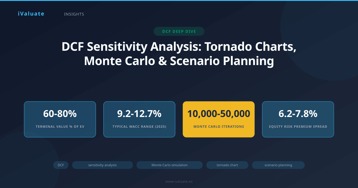
Recent market data illustrates this challenge acutely. In Q4 2024, the median WACC for software companies ranged from 9.2% to 12.7% depending on size, profitability, and leverage—a 380 basis point spread that translates to valuation differences of 25-40% for the same cash flow profile. For private equity firms evaluating platform acquisitions or corporate development teams assessing strategic targets, understanding this sensitivity is not academic—it directly impacts bid strategy, financing structure, and deal approval.

The Professional Standard: Multi-Dimensional Sensitivity

Best-in-class valuation practices now require three layers of sensitivity analysis:

One-way sensitivity tables: Isolating individual variables (WACC, terminal growth, revenue CAGR) to show their isolated impact on enterprise value
Two-way sensitivity matrices: Examining the interaction between paired variables, typically WACC and terminal growth or revenue growth and EBITDA margin
Scenario-based analysis: Developing coherent base, bull, and bear cases with internally consistent assumption sets

These approaches serve different analytical purposes and audiences. One-way tables help identify which assumptions matter most. Two-way matrices reveal interaction effects and non-linear relationships. Scenario analysis provides narrative context that resonates with non-technical stakeholders.

02 Tornado Charts: Visualizing Relative Impact

The tornado chart—named for its distinctive shape—ranks input variables by their impact on valuation, displaying them in descending order of influence. This visualization immediately answers the critical question: "Which assumptions drive the most valuation uncertainty?"

Construction Methodology

To build a tornado chart, each input variable is flexed independently while holding all others constant at their base case values. The typical approach:

Define a reasonable range for each variable (e.g., ±10% for operating assumptions, ±100-200 bps for discount rates)
Calculate enterprise value at the high and low end of each range
Measure the total valuation swing (high case minus low case)
Rank variables by the magnitude of this swing
Display horizontally with the base case as the central axis

For a $650 million industrial distribution business valued in early 2025, a tornado analysis revealed the following sensitivity ranking:

WACC (8.5% to 10.5%): $582M to $728M (±$73M swing)
Terminal EBITDA margin (11.5% to 13.5%): $598M to $702M (±$52M swing)
Terminal growth rate (2.0% to 3.0%): $612M to $688M (±$38M swing)
Revenue CAGR Years 1-5 (3.5% to 5.5%): $628M to $672M (±$22M swing)
Working capital intensity (8% to 12% of revenue): $638M to $662M (±$12M swing)

This analysis immediately clarifies that discount rate assumptions and terminal profitability drive far more valuation uncertainty than near-term revenue growth or working capital efficiency. For the acquiring company, this insight shifted due diligence focus toward validating sustainable margin assumptions and refining cost of capital estimates rather than debating Year 2 revenue projections.

Professional Application Guidelines

Effective tornado charts require thoughtful parameter selection. The ranges chosen must be:

Realistic: Based on historical volatility, industry benchmarks, or management guidance ranges
Consistent: Using comparable confidence intervals (e.g., 80% confidence or ±1 standard deviation) across variables
Material: Focusing on 6-10 key drivers rather than exhaustively testing every model input

In the current market environment, WACC sensitivity deserves particular attention. With the 10-year Treasury fluctuating between 4.2% and 4.8% in Q1 2025, and equity risk premiums varying by sector (technology: 7.2%, healthcare: 6.8%, industrials: 6.4%), even sophisticated practitioners face 150-250 basis points of reasonable WACC uncertainty for middle-market companies.

03 Spider Diagrams: Mapping Multi-Variable Scenarios

While tornado charts examine variables in isolation, spider diagrams (also called sensitivity spiders or scenario webs) visualize how multiple assumptions move together under different scenarios. This approach acknowledges that real-world outcomes involve correlated changes across multiple inputs.

Scenario Architecture

Professional spider diagrams typically incorporate three to five scenarios:

Base Case: Management's most likely forecast, validated against industry benchmarks and historical performance. For a SaaS company in 2025, this might assume 22% ARR growth, 78% gross retention, 25% Rule of 40 score, and 10.2% WACC.

Bull Case: Optimistic but achievable outcomes, often representing 75th-80th percentile performance. Variables move favorably in concert—higher growth coincides with improving unit economics and multiple expansion. The same SaaS company might model 32% ARR growth, 82% gross retention, 35% Rule of 40, and 9.4% WACC (reflecting lower perceived risk).

Bear Case: Downside scenario reflecting operational challenges, market deterioration, or competitive pressure. Variables deteriorate together—slower growth, margin compression, higher discount rates. Here: 12% ARR growth, 72% gross retention, 15% Rule of 40, and 11.8% WACC.

Some practitioners add "Management Case" (often more optimistic than base) and "Stress Case" (worse than bear, testing covenant compliance or solvency).

Visual Construction

The spider diagram plots each scenario as a line radiating from a central point, with axes representing different input variables normalized to their base case values (typically set at 100%). The resulting web-like pattern shows how scenarios diverge across multiple dimensions simultaneously.

For a $280 million consumer products acquisition evaluated in late 2024, the spider diagram revealed an important insight: the bull and bear cases diverged most significantly on terminal value assumptions (±35% from base) and EBITDA margin trajectory (±28%), while near-term revenue growth showed relatively tight clustering (±12%). This pattern indicated that the investment thesis hinged primarily on long-term competitive positioning and operational improvement rather than market growth rates—a finding that shaped post-acquisition value creation planning.

Correlation Considerations

Sophisticated spider analysis incorporates realistic correlation structures. Revenue growth and EBITDA margins often exhibit negative correlation in the short term (growth investments pressure margins) but positive correlation long-term (scale drives efficiency). Discount rates and growth rates typically move together (stronger growth environments coincide with lower risk premiums).

Ignoring these correlations produces scenarios that are internally inconsistent and analytically misleading. A scenario combining 35% revenue growth with 200 basis points of margin expansion and a 12% WACC is likely incoherent—exceptional growth rarely coincides with elevated risk premiums in efficient markets.

04 Monte Carlo Simulation: Quantifying Probability Distributions

Monte Carlo simulation represents the most sophisticated approach to DCF sensitivity analysis, generating thousands of valuation outcomes by randomly sampling from probability distributions assigned to each input variable. Rather than discrete scenarios, Monte Carlo produces a continuous probability distribution of enterprise values.

Technical Implementation

The Monte Carlo process involves five steps:

1. Identify key variables: Typically 8-15 inputs that drive material valuation uncertainty (revenue growth rates, margin assumptions, WACC components, terminal value parameters).

2. Define probability distributions: For each variable, specify the distribution type (normal, lognormal, triangular, uniform) and parameters (mean, standard deviation, min/max bounds). Revenue growth might follow a normal distribution with mean 4.5% and standard deviation 2.1%, while WACC might use a triangular distribution bounded by 8.5% (minimum), 10.2% (most likely), and 12.5% (maximum).

3. Specify correlations: Build a correlation matrix reflecting historical relationships or economic logic. In 2024-2025 market data, revenue growth and equity risk premiums showed -0.42 correlation for cyclical industries, while terminal growth and long-term inflation expectations exhibited +0.67 correlation.

4. Run iterations: Execute 10,000-50,000 simulations, each drawing random values from the specified distributions while respecting correlation constraints, calculating enterprise value for each iteration.

5. Analyze results: Examine the distribution of outcomes, calculating percentiles, confidence intervals, and probability of achieving specific thresholds.

Real-World Application: Healthcare Services Platform

A private equity firm evaluating a $520 million healthcare services platform in Q1 2025 employed Monte Carlo simulation with the following parameter structure:

Revenue CAGR (Years 1-5): Normal distribution, mean 6.8%, σ = 2.4%
EBITDA margin (Year 5): Triangular distribution, min 16.5%, mode 18.2%, max 20.5%
WACC: Triangular distribution, min 9.2%, mode 10.4%, max 12.1%
Terminal growth: Normal distribution, mean 2.8%, σ = 0.8%, truncated at 1.5%-4.0%
Capex intensity: Uniform distribution, 3.5%-5.5% of revenue

After 25,000 iterations, the simulation produced these results:

Mean enterprise value: $518 million
Median enterprise value: $512 million
Standard deviation: $94 million
10th percentile: $392 million
90th percentile: $658 million
Probability of value exceeding $600M: 18.3%
Probability of value below $450M: 24.7%

The distribution exhibited slight positive skew (mean > median), reflecting the asymmetric impact of terminal value assumptions—upside scenarios benefit disproportionately from higher terminal multiples and growth rates.

This probabilistic framework enabled sophisticated decision-making. The firm structured its bid at $485 million (55th percentile outcome), providing 27 million of downside buffer to the median while remaining competitive. The analysis also informed earnout structuring, with performance thresholds set at the 65th percentile outcome ($540 million value realization) to align management incentives with above-median performance.

Distribution Selection Principles

Choosing appropriate probability distributions requires both statistical rigor and business judgment:

Normal distributions suit variables with symmetric uncertainty and no hard bounds—revenue growth rates, inflation assumptions, or margin changes often fit this pattern.

Lognormal distributions apply to variables that cannot go negative and exhibit right skew—equity risk premiums, volatility measures, or commodity prices frequently follow lognormal patterns.

Triangular distributions work well when you have minimum, maximum, and most likely estimates but limited historical data—useful for terminal value assumptions or new market penetration rates.

Uniform distributions represent maximum uncertainty within defined bounds—appropriate when all values in a range are equally likely, such as regulatory approval timing or contract renewal rates with limited precedent.

05 Integrating Sensitivity Analysis into Investment Decisions

The value of sophisticated sensitivity analysis lies not in the elegance of the mathematics but in its impact on decision quality. Three practical applications demonstrate this principle:

Deal Structuring and Negotiation

Understanding valuation sensitivity enables creative deal structures that bridge valuation gaps. When a strategic acquirer and founder-owner disagreed on the value of a specialty manufacturing business in late 2024—the buyer's DCF indicated $175 million while the seller sought $210 million—tornado analysis revealed that 60% of the disagreement stemmed from differing terminal EBITDA margin assumptions (buyer: 14.2%, seller: 16.8%).

The solution: a two-year earnout tied to EBITDA margin achievement, with $180 million paid at close and up to $25 million contingent on reaching 16%+ margins by Year 2. The structure converted valuation uncertainty into aligned incentives, facilitating transaction completion.

Risk Management and Covenant Compliance

Lenders and credit committees increasingly demand sensitivity analysis to assess downside scenarios and covenant headroom. A $350 million leveraged buyout in the business services sector used Monte Carlo simulation to demonstrate that even at the 25th percentile outcome, the company would maintain 1.8x interest coverage and 4.2x net leverage—comfortably above covenant thresholds of 1.25x and 5.5x respectively.

This analysis supported approval of a more aggressive capital structure (5.8x total debt/EBITDA) than traditional deterministic modeling would have permitted, reducing equity contribution requirements by $45 million.

Portfolio Management and Capital Allocation

For corporate development teams managing acquisition pipelines, comparing spider diagrams across opportunities reveals which investments offer superior risk-adjusted returns. A diversified industrial company evaluating three bolt-on acquisitions in Q4 2024 used standardized sensitivity analysis to compare opportunities:

Target A: Narrow valuation range ($82M-$118M, 80% confidence), low sensitivity to macro assumptions, limited upside
Target B: Wide range ($65M-$155M), high WACC sensitivity, significant operational leverage
Target C: Moderate range ($94M-$136M), balanced sensitivity profile, strong strategic fit

The company prioritized Target C, recognizing that Target A offered insufficient upside to justify integration complexity while Target B's volatility created unacceptable risk given the company's leverage constraints.

06 Technical Considerations and Common Pitfalls

Implementing sophisticated sensitivity analysis requires attention to several technical challenges:

Assumption Independence vs. Correlation

Tornado charts assume variables move independently—a simplification that can mislead. In reality, revenue growth, margins, and discount rates exhibit complex correlations. Monte Carlo simulation addresses this through correlation matrices, but practitioners must validate that specified correlations reflect economic reality rather than spurious historical relationships.

Terminal Value Dominance

In typical DCF models, terminal value represents 60-80% of enterprise value for growth companies. This concentration means terminal value assumptions (growth rate, exit multiple, terminal margin) drive disproportionate sensitivity. Some practitioners address this by running separate sensitivity analyses for the explicit forecast period and terminal value, then combining results.

Discrete vs. Continuous Distributions

Real-world outcomes often involve discrete events (regulatory approval/rejection, contract win/loss, market entry success/failure) that don't fit continuous probability distributions. Hybrid approaches combine scenario analysis for discrete events with Monte Carlo simulation for continuous variables, though this adds modeling complexity.

Computational Intensity and Model Transparency

Monte Carlo simulation with 25,000+ iterations can strain complex Excel models, requiring VBA programming or specialized software. This creates a tension between analytical sophistication and model transparency—simpler models are easier to audit and explain but may sacrifice realism.

Professional valuation platforms like iValuate address this challenge by combining computational power with intuitive interfaces, enabling sophisticated sensitivity analysis without sacrificing accessibility or auditability.

07 Presenting Results to Different Audiences

The most sophisticated analysis fails if poorly communicated. Effective presentation adapts to audience sophistication:

For boards and senior executives: Lead with scenario analysis (base/bull/bear) presented in simple tables showing enterprise value, implied equity value per share, and key return metrics (IRR, MOIC). Follow with a single tornado chart highlighting the top five value drivers. Avoid statistical jargon; focus on business implications.

For investment committees and credit committees: Present comprehensive two-way sensitivity matrices for critical variable pairs (WACC vs. terminal growth, revenue CAGR vs. terminal margin). Include Monte Carlo results showing probability distributions and percentile outcomes. This audience appreciates technical rigor and wants to understand tail risks.

For operating management: Emphasize spider diagrams that show how operational levers (margin improvement, revenue growth, working capital efficiency) translate to value creation. Connect sensitivity analysis to strategic initiatives and performance targets. Management teams respond to frameworks that link their decisions to valuation outcomes.

For external stakeholders (lenders, minority investors): Focus on downside protection and covenant compliance. Present stress scenarios and show how the investment performs under adverse conditions. This audience prioritizes risk mitigation over upside potential.

08 The Evolution of Sensitivity Analysis in 2025-2026

Several trends are reshaping how professionals approach DCF sensitivity analysis:

Integration with real options analysis: For companies with embedded optionality—expansion opportunities, abandonment flexibility, or strategic pivots—traditional sensitivity analysis is being supplemented with real options frameworks that explicitly value managerial flexibility.

Machine learning-enhanced distributions: Rather than assuming normal or triangular distributions, some practitioners are using historical data and machine learning algorithms to derive empirical distributions that better capture fat tails and asymmetric risks.

Dynamic scenario updating: As new information emerges during due diligence or post-acquisition, leading firms update probability distributions and rerun simulations in real-time, treating valuation as a continuously refined estimate rather than a static conclusion.

ESG integration: Environmental, social, and governance factors are being incorporated into sensitivity analysis through scenario planning (carbon pricing scenarios, regulatory change cases) and as discrete variables in Monte Carlo frameworks (probability of ESG-related disruption, impact on cost of capital).

09 Conclusion: From Precision to Confidence

The shift from point estimates to probabilistic valuation represents a maturation of the profession. In an environment where the S&P 500 traded in a 4,200-4,800 range during 2024, where WACC assumptions for middle-market companies span 300+ basis points, and where terminal value assumptions can swing valuations by 40-60%, pretending that DCF analysis produces precise answers is professionally indefensible.

Tornado charts, spider diagrams, and Monte Carlo simulation transform DCF from a false precision exercise into a framework for understanding uncertainty, identifying key value drivers, and making better decisions under ambiguity. These tools don't eliminate uncertainty—they quantify it, visualize it, and make it manageable.

The most successful valuation professionals in 2025 recognize that their role is not to predict the future with spurious accuracy but to map the range of plausible futures and help stakeholders navigate that landscape. Whether supporting a $50 million bolt-on acquisition or a $5 billion strategic merger, the analytical frameworks remain consistent: identify what matters, quantify the uncertainty, and communicate the implications clearly.

For firms seeking to implement these sophisticated approaches efficiently, modern valuation platforms like iValuate provide the computational infrastructure and visualization tools that make advanced sensitivity analysis accessible without requiring custom programming or sacrificing model transparency. As markets remain volatile and stakeholders demand greater analytical rigor, the ability to present DCF results with comprehensive sensitivity analysis has evolved from a competitive advantage to a professional imperative.

DCF Sensitivity Analysis: Tornado Charts, Monte Carlo & Scenario Planning